
Multi-scale Feature Learning Dynamics: Insights for Double Descent
What is double descent?
One of the very first concepts that I learned in Machine Learning was the bias/variance trade-off meaning that the generalization curve is U-shaped. According to statistical learning theory, a small model under-fits, a reasonably-sized model fits just right, and a large model should over-fit.
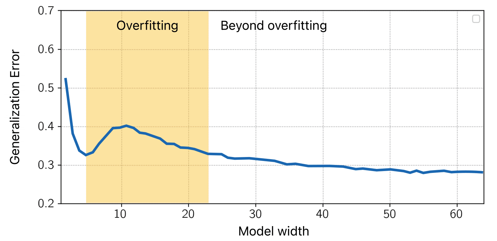
However, that doesn't seem to be the case! Below, we have a ResNet18 trained on Cifar-10. In contrast to classical wisdom, increasing the model-size, beyond the overfitting regime, results in a second descent of the generalization error. [Belkin et al.] calls this behavior "the double descent".
More recently, [Nakkiran et al.] reported that if we let the x-axis denote the training time (epochs), a similar double descent occurs, which is referred to as “the epoch-wise double descent”. Let’s look at an interesting experiment in [Nakkiran et al.] that visualizes the interplay between the regularization strength and training time.

The above figure is a classification task on Cifar-10 using a large ResNet18.
Left graph: The color shades show the generalization. Yellow
- For a model with
low complexity , we can see that it starts with a large error, and as we train more, the generalization error decreases. - For a model with
intermediate levels of complexity , the generalization curve follows the classical U-shaped curve. - Interestingly, models with higher
levels of complexity exhibit an epoch-wise double descent curve.
It is pretty clear that there are things that we do not fully understand about generalization in high-dimensional statistics. In this work, we investigate the reasons underlying such generalization behavior.
A Teacher-Student Framework
Here, we introduce a model that,
- is complex enough to exhibit epoch-wise double descent, and yet,
- is simple enough that it allows for analytical study.
To that end, we consider a linear teacher-student setup, where,
- The teacher plays the role of the data generating process, and,
- The student learns from the data generated by the teacher.
As shown in the diagram at the beginning of this post, a teacher generates pairs of \((x, y)\) from which the student learns.
An important remark here is that the matrix \(F\) modulates the student's access to latent features \(z\). The idea behind the matrix \(F\) is to simulate multi-scale feature learning similar to that of neural networks. Particularly, the condition number of \(F\) determines how much faster some features are learned than others. Similarly, in neural networks on vision tasks, it is well-known that, for example, color and texture are learned faster than more complex shape features.
In such a teacher-student setup,
- A condition number of
\(\kappa=1\) means that all the features are learned at the same rate. - A
\(\kappa=100\) means that the fastest learning subset of features are learned 100x faster than the slowest. (double descent is observed) - A
\(\kappa=100000\) means that a subset of features is so slow that they do not get learned at all. (traditional U-shaped)

To understand what is going on, we take a closer look at the generalization error.
We show that using the replica method of statistical physics [Engel & Van den Broeck], the generalization error can be derived analytically, such that,
$$\mathcal{L}_G = \frac{1}{2}(1 + Q - 2R)$$
where \(\mathcal{L}_G\) is the generalization error and \(R\) and \(Q\) are defined as,
$$R := \frac{1}{d}{W^*}^TF\hat{W}, \qquad \qquad Q := \frac{1}{d}\hat{W}^TF^TF\hat{W}.$$
Both \(R\) and \(Q\) have clear interpretations; \(R\) is the dot-product between the teacher's weights \(W\) and the student's
We encourage interested readers to visit the main paper in which we derive closed from expressions for \(R(t, \lambda)\) and \(Q(t, \lambda)\), describing their dynamics as a function of training time \(t\) and the regularization coefficient \(\lambda\). The take-home message is that R and Q can be decomposed into two components: A fast-learning component, and a slow-learning component. Essentially, as the fast-learning features overfit, slower-learning features start to fit, resulting in a second descent in test error (Eqs. 11-15 of the paper).
Now, recall the earlier heatmap plot we presented for a ResNet-18 on Cifar-10. We can plot the same heatmap but for our linear teacher-student model and using analytical expression:

A qualitative comparison shows a close match between the two! It is observed that in both experiments, a model with intermediate levels of regularization displays a typical overfitting behavior where the generalization error decreases first and then overfits. This is consistent with the common intuition that larger amounts of regularization act as early stopping. Put differently, learning of slow features requires large weights, which is penalized by the weight-decay. On the other hand, a model with a smaller amount of regularization exhibits the double descent generalization curve.
What comes next?
This blog post studied epoch-wise double descent by leveraging the replica method from statistical physics to characterize the generalization behavior using a set of informative macroscopic parameters (namely, R and Q). Crucially, these quantities can be used to study other learning dynamics phenomena and offer the possibility to be monitored during training, allowing a useful dichotomy of a model's key features influencing generalization. A future direction to study the generalization dynamics in cases where the first descent is so significant that the training loss decreases to very small values; So small that, either,
- learning slower features becomes practically impossible due to the Gradient Starvation phenomenon [Pezeshki et al.], or
- learning happens after a very large number of epochs. Such behavior, referred to as Grokking [Power et al.], is a phenomenon in which the model abruptly learns to generalize perfectly but long after the training loss has reached very small values.
Finally, while our simple teacher-student setup exhibits certain intriguing phenomena of neural networks, its simplicity introduces several limitations. Studying finer details of the dynamics of neural networks requires more precise, non-linear, and multi-layered models, which introduce novel challenges that remain to be studied in future work.